Topics:
- Identifying and installing actuators for the engine management system
- Fuel injectors
- Selecting suitable injectors
- Mounting injectors in the intake manifold
- Ignition
- Preparing with conventional ignition
- Coil for the engine management system
- Current build-up in the primary coil
- Ignition timing advance
- Throttle body
- Stepper motor test setup with simulator
- Stepper motor settings
- Fuel pump circuit
- Completing mechanical work
Identifying and installing actuators for the engine management system:
The actuators to be controlled by the MegaSquirt are the injectors, coil, fuel pump, and the idle speed stepper motor. This chapter describes the process of testing and mounting these actuators on the engine block, and the choices made in this regard.
Fuel injectors:
The MegaSquirt controls the injectors. The injectors are ground-switched. In a ground-switched component, power is present, but current only flows when the ground is activated. In this case, the injector will only spray when the MegaSquirt ECU switches the ground. Once the energization is terminated, the injector stops spraying. The amount of fuel to be injected is determined based on the VE table and AFR table.
A MOS-FET switches the injector on and off to inject the fuel. The amount of fuel determined by the MegaSquirt depends on several factors:
- The ideal gas law relating the amount of air to its pressure, volume, and temperature;
- Measured values by sensors in the engine block: manifold pressure (MAP sensor), coolant and intake air temperature, crankshaft speed, and throttle position sensor data;
f Adjustment parameters: required fuel quantity, volumetric efficiency (VE), injector opening time, and enrichment under certain conditions.
Injection time should be as long as possible during engine idle to achieve good fuel dosing. Therefore, any injector cannot just be applied to the engine without consideration. The properties of different types of injectors must be compared, and calculations should provide insight into the required fuel quantity for the respective engine. A choice was also possible between high and low impedance injectors. Low-impedance injectors are suitable for engines where very fast opening of the injector needle is required, typically having a resistance of 4 Ohms. The disadvantage of these injectors is the high current. The resulting heat development in the MegaSquirt is undesirable. It is possible to use low-impedance injectors by mounting special IGBTs on a heat-conducting plate on the MegaSquirt housing. The choice was made to use high-impedance injectors to minimize heat development, thus not utilizing these IGBTs.
The flow rate is crucial in determining the correct injection amount, and thus the control. Choosing injectors that are too large will result in a very short injection time at idle speed, potentially causing irregular engine running. The injection quantity must be enough to inject all fuel in the available time. The injection amount is indicated as injection time in milliseconds, based on high load and high engine speed at a MAP of 100 kPa. Based on engine properties, the required injector flow can be calculated, indicating how many milliliters of fuel are injected per minute.
Selecting the suitable injectors:
For the project, injectors of three different types were provided. Research determined which type of injector was most suitable for this project.
Each type of injector has a different flow rate; the output after a minute of injecting varies by type. Before testing the injectors, they underwent cleaning in an ultrasonic bath. This cleaning method uses ultrasonic waves and a special test fluid to clean the injector inside and out, ensuring any old residues do not affect the flow measurement or spray pattern. During ultrasonic cleaning, the injectors were continuously opened and closed, and the spray pattern of each injector was observed as a fine mist. No abnormalities such as droplet formation or an irregular stream were seen upon closure. After ultrasonic cleaning and testing, the O-rings were replaced to ensure a good seal when mounted in the intake manifold.
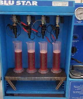
Using a test setup (see above image), injectors can spray into multiple measuring cups, allowing the sprayed fuel amount to be read after a certain time. By controlling the injectors at an operating pressure of 3 bar, the injected fuel amount can be verified. The fuel pressure on the supply line (the rail) should be 3 bar, and the injector needle must be controlled with a 100% duty cycle for 30 or 60 seconds. After the injectors were controlled for 30 seconds, the following data could be filled in:
Type 1: 120 ml
Type 2: 200 ml
Type 3: 250 ml
Only one type of injector will be used. The injector size is determined using the formula below:
The injector size is determined based on the effective power (Pe) delivered at a certain speed, the Break Specific Fuel Consumption (BSFC), the number of injectors (n injectors), and the maximum duty cycle with which the injectors are controlled. The result is multiplied by 10.5 to convert from pounds per hour (lb/hr) to ml/min.
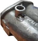
The calculation result indicates which injector is suitable for this engine configuration. A deviation of less than 20 ml from the calculated value is not problematic. This difference is compensated by adjusting the MegaSquirt software. The following table provides an overview of the data used in the formulas:
The first step is to determine the fuel injected at the torque speed. A certain amount of air is drawn in per two crankshaft revolutions. At torque speed, volumetric efficiency is highest. Due to the engine’s properties (including valve overlap), the engine fills best at this speed, and efficiency is highest. Volumetric efficiency is estimated at around 70%. Formula 4 calculates the air volume present in the engine at that moment.
In formula 5, the amount of fuel injected is calculated based on the present air volume. The engine power achieved at torque speed is calculated in formula 6. The ratio between the injected fuel quantity and power is indicated by BSFC in formulas 7 and 8.
The actual BSFC is multiplied by 3600 in formula 6 to convert to kWh. The BSFC of a gasoline engine usually ranges between 250 and 345 g/kWh. The lower the value, the more efficient the engine is. Formula 8 indicates the ratio between fuel flow in pounds per hour and effective engine power. This percentage is used in formula 9.
The answer from formula 9 clarified that injectors with a flow of 200 ml/min are suitable for the engine. The 7 ml difference is negligible as it is compensated in the software by adjusting the VE table.
Mounting injectors in the intake manifold:
The electronically controlled injection system allows for the removal of the carburetor, which was part of the classic setup. The carburetor is thus replaced with a throttle body (for air supply) and four separate fuel injectors. The intake manifold was retained and modified to enable the conversion to the engine management system. Fuel injection occurs in the intake manifold. The choice was made to mount the injectors as close as possible to the intake valve. Engine constructors often mount the intake valve under an angle in the intake manifold. Fuel is then sprayed against the intake valve. However, in the current project, the injectors are placed at a 45-degree angle relative to the air channels in the manifold.
The intake manifold is made of cast aluminum. Aluminum bushings were chosen to be attached to the manifold. Manually machining to the correct size was not an option, as the bushings needed non-standard dimensions compared to any drill size. This meant outsourcing the bushings to a company with suitable equipment. The bushings were then attached to the manifold using TIG welding. The decision to mount the injectors upright instead of at an angle was made for the following reason:
- The mounting process: it’s easier to arrange the bushings in a straight, horizontal setup. Welding the bushings to the manifold is simpler as now it can be easily welded around, unlike when the bushing is at an angle.
- The post-processing: During welding, the bushings become slightly oval. This deformation results from the heat during the welding process. This was considered by making the inner diameter of the bushings smaller than the injectors’ outer diameter. Post-processing (reaming) is less risky: when the bushings are round again inside, the diameter is optimal for the injectors, ensuring the O-rings maintain the seal. The bushings’ height is crucial; the injector must not be inserted too far into the manifold. The injector’s end shouldn’t obstruct the airflow. Based on information from the source: (Banish, Engine Management, advanced tuning, 2007), it’s decided to mount the injectors deep enough in the manifold that the ends are precisely in the manifold holes; the airflow isn’t hindered.
- Fuel injection: Since the fuel mist’s mixing with the air is optimal before the intake valve opens, it doesn’t matter much whether the injector sprays directly on the intake valve or just before in the intake manifold.
In simultaneous injection, injection occurs every crank rotation (3600). All four injectors spray simultaneously. This also means fuel is sprayed into the intake port while the intake valve isn’t open. Sometime later, the intake valve opens, and the fuel enters the cylinder.
The bushings were custom-sized on a lathe. The inner diameter is slightly smaller than the injector’s outer diameter; because deformation occurs during welding, there’s room for material removal during post-processing. The diameter slightly enlarges as material is removed. The diameter mustn’t be too large, as the rubber O-ring on the injector might not seal well enough. A good seal is essential; air leakage along the injector results in reduced manifold vacuum.The measured vacuum then no longer matches the calculated vacuum. This affects the injection determined based on the VE table. The vacuum is a significant factor. The VE table’s features and settings are described in the following chapter.
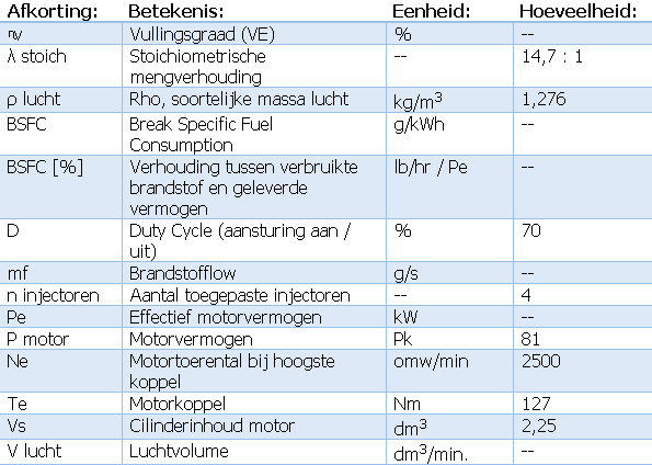
A chamfer was filed at the bottom of the bushings so they match the intake manifold’s shapes. The bushing must stand as straight as possible. The image below shows the intake manifold with a bushing during assembly. The bushing is tacked on one side, allowing observation of welding’s effect on the material. It was unclear whether the intake manifold’s aluminum contained too many impurities that might complicate welding. This wasn’t the case. To prevent bushings from shifting during welding, holes were pre-drilled in the manifold, and the bushings were positioned correctly with a specially-fabricated jig. This way, the four bushings were securely welded around. A final check showed the joints between the bushings and the manifold were airtight.
The connection between the injectors is usually formed by a solid injector rail. This aluminum alloy tube with fittings is precisely crafted by a constructor. In the Land Rover engine used for the project, there are two injectors adjacent to each other, but the space between injector pairs is quite large. The dimensions of the fuel rail and the space between the air channels in the intake manifold didn’t match, necessitating rail modification.
Shortening some sections and extending others through soldering is challenging; impurities from old fuel, difficult to remove from inside the rail, can deteriorate solder adhesion. Because it involves fuel, the safest method was chosen; the parts to which the injectors are attached were connected with high-quality fuel hoses. All ends have flared edges, and sturdy hose clamps are applied to prevent hose slippage over the flares.
The image below shows the intake manifold during processing. The supply line (marked with number 1) is connected to the fuel pump’s output. Fuel is supplied under 3 bar pressure at the inlet of the four injectors. The pressure regulator (3) adjusts the pressure based on manifold pressure, as the pressure difference between fuel pressure and manifold vacuum should remain at 3 bar. Fuel circulates back to the tank via the return line (2). Continuous fuel circulation occurs. Only when the injectors are controlled by the MegaSquirt ECU does injection take place.
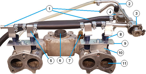
- Supply line
- Return line
- Pressure regulator
- Pressure check
- Heat shield
- Throttle connection
- Vacuum connection
- Injector cylinder 1
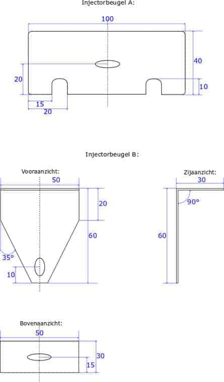
- Injector bracket A
- Injector bracket B
- Intake port cylinder 1
In existing passenger vehicles, injector rails are usually clamped to the intake manifold using clamps or eyelets. The injector rail then clamps the injectors into the manifold. For this project, a flexible fuel hose was chosen for the injector rail, making the earlier mentioned method impossible. Therefore, the injectors are clamped into the intake manifold using a custom bracket. The brackets consist of two parts: an upper part (bracket A) and a lower part (bracket B).
Bracket A has two notches that can slide over the injectors. This presses the injectors against the manifold using the flat sides. Slots in both brackets A allow adjustment of the distance the injectors sit in the slots. Brackets A and B are screwed together. Bracket B is attached to the same stud that mounts the manifold to the engine. A slot allows vertical adjustment of the bracket. Moving the bracket downward increases how tightly the injector is clamped.
Ignition:
The conventional ignition was replaced by an electronically controlled ignition system with a coil controlled by the MegaSquirt. Initially, the original system with contact points must be connected to ensure the engine functions fully on original techniques. After several hours of operation can it be determined that the engine is functioning properly, allowing for installation and adjustment of, among other things, the electronic ignition.
Preparing with conventional ignition:
The Land Rover engine was originally equipped with an ignition system with contact points, now commonly referred to as a conventional ignition system. The image shows this type of ignition system.
With closed contact points, the primary current begins to build. The current is limited to 3 to 4 Amps by the primary coil’s resistance. When a current flows through the coil’s primary coil, a magnetic field is built. Both the primary (3) and secondary coil (4) are in this magnetic field. When the current through the contact points (10) is interrupted by the breaker cam (9) on the distributor shaft, voltage is induced in both coils. About 250 volts arise in the primary coil. The difference in turns will induce a voltage of 10 to 15 kV in the secondary coil. A spark plug spark occurs when the points open.
Induction voltage can be limited by allowing the primary current to continue momentarily after the contact points open. This is achieved with a capacitor connected parallel to the contact points. The capacitor acts as a time-determining element that, depending on its capacity, regulates the induction voltage height. It also prevents contact points from burning.
Coil for the engine management system:
The engine management system will control the coil. The classic coil with distributor will remain on the engine as a test setup but no longer plays a part in the combustion engine’s operation. A Distributorless Ignition System (DIS coil) was chosen, translated as “distributorless ignition system.” This type of ignition system does not use a distributor. Another option was to choose a Coil On Plug (COP) coil, which attaches a separate coil to each spark plug. A COP coil is also called a pen coil. The disadvantage of a COP coil is less efficient heat dissipation compared to a DIS coil. Applying COP coils also requires a camshaft sensor signal, which is not present on the current engine.
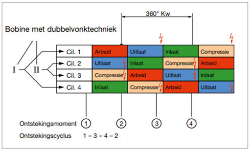
The missing tooth on the crankshaft pulley serves as the reference point for determining the ignition timing. With the DIS coil, two spark plugs will be controlled simultaneously at one ignition moment. The DIS coil is essentially a unit with two coils installed. When the pistons of cylinder 1 and 4 move upwards, one is undergoing a compression stroke while the other is on an exhaust stroke. Yet both spark plugs spark. The spark in the cylinder undergoing the compression stroke ignites the mixture. The other spark, the so-called “wasted spark,” sparks while the exhaust gas leaves the combustion chamber. The wasted spark forms when no mixture is ignited. Its ignition energy is low; despite the spark, energy loss is minimal. It is also not harmful.
The image shows the working diagram of a four-cylinder petrol engine with a DIS coil. This diagram shows two ignition markings per ignition moment; one generates the spark to ignite the mixture, the other is the wasted spark. A DIS coil can be controlled with just two pulses by the MegaSquirt.
When cylinder 1 undergoes a compression stroke and cylinder 4 an exhaust stroke, the MegaSquirt controls the primary coil A via pin 36 on DB37 (see image below). This control is based on the crankshaft reference point (between 90 and 120 degrees before TDC). The MegaSquirt controls primary coil B, responsible for spark formation in cylinders 2 and 3, 180 degrees after coil A. No reference point is present for coil B, but ignition timing can be simply determined by counting teeth on the 36-1 trigger wheel.
Between coil A and pin 7 of the processor is a 330-ohm resistor depicted. This resistor limits the drive pulse’s current and induced voltage. As this resistor is not standard on the MegaSquirt circuit board, it must be mounted afterward. Components left of the vertical dashed line in the image below show the internal circuit of the MegaSquirt. The components shown (two 330 ohm resistors and LEDs) were to be soldered onto the circuit board afterward.
Current build-up in the primary coil:
It is important to understand the current build-up in the primary coil. Besides the current strength, the coil’s charging time can also be determined. Charging time depends on several factors that the MegaSquirt must account for.
The self-inductance coefficient (L-value) of the chosen coil is 3.7mH. Combined with the ohmic resistance R, the maximum primary current and curve rise time are determined. A small L-value and resistance result in a fast current rise after activation. With the known coil data, primary current build-up can be calculated.
The following formula shows the general solution to the first-order differential equation, calculating current strengths, charge, and discharge times to display the switching phenomenon using a curve.
The equation is:
where the time constant (Tau) is calculated:
The maximum current, according to Ohm’s Law, would be 28 Amps:
In reality, this current strength won’t be achieved.
The coil is turned off sooner. The reason is explained later. Filling in this data in the general formula gives:
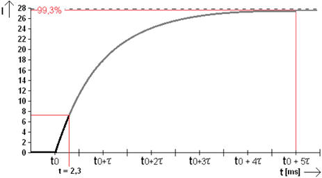
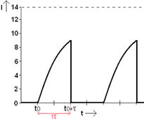
The image shows the charging curve of the primary coil. From time T0 to 1 Tau, the coil is 63.2% charged. This is a fixed percentage for coil charging time. Formula 13 shows the coil is charged to 17.7 Amps at 1 Tau. At t = 5 Tau, the end value is practically reached.
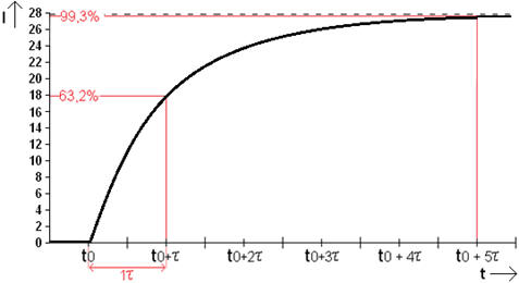
According to coil specifications, the primary current after charging amounts to 7.5 A. The current doesn’t rise higher. Time to reach 7.5 A is called dwell time, depending on battery voltage, here 14 volts. Without regulating, the coil current would, according to formula 12, max out at 28 Amps.
The coil according to formula 14 is charged to 17.7 A at t = 7.4 ms. Actual charging time is shorter since the coil maxes at 7.5 A. Required time can be calculated using known data in formula 15.
Primary current build-up stops at 7.5 A. This prevents excessive and unnecessary coil heating. The crucial factor is optimally charging the coil in the shortest possible time. The image shows the charge curve to t = 2.3 ms.
When battery voltage drops, for example, during engine starting, it affects dwell time. It takes longer than 2.3 ms to reach 7.5 A. The previously known formula determines new charge time. Maximum current is determined by battery voltage:
The charge time to 7.5 A with a maximum of 20 A is calculated in formula 17:
In the image, charge time at 14 volts is shown with the black line, and at 10 volts with green. Both lines fall to zero at the same moment: the ignition timing. At lower battery voltage, more time is needed to charge the primary coil; therefore, the MegaSquirt must activate primary current earlier.
The black lines (rising and falling) indicate dwell time at 14 volts. The green line shows advanced charge time at lower voltage: this is 94t. Therefore, actual charge time is 94t + 100%.
Later in this paragraph, this is clarified with an example and figure 36. Charging time is extended, and ignition timing remains the same. Failure to do so sufficiently affects the energy released during ignition. The primary current would switch off too early, preventing the 7.5 A current strength from being reached. Lengthening primary coil charging time (dwell time) is a function of battery voltage. Calculating dwell time for various voltages yields different maximum coil current strengths.
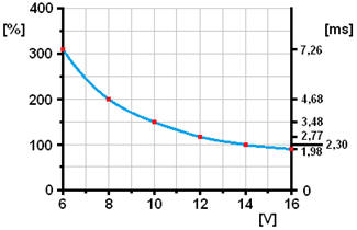
Assuming battery voltage can drop to 6 volts during starting and rise to 14.7 volts during charging, a curve can be sketched by calculating intermediate values. The image below shows dwell time correction for the applied DIS coil. For every 2 volt increase, a (red) point is placed on the graph. An earlier entered dwell time of 2.3 ms at 14 volts in the TunerStudio program serves as the starting point, forming a correction factor above this voltage. A voltage of 14 volts is therefore 100% (no correction).
Now it is apparent that charging time increases up to 315% at 6 volt battery voltage.
Battery voltage can drop to 6 volts under adverse conditions, leading to a weakened ignition spark. Extending dwell time (the time primary current flows) compensates for this, ensuring adequate ignition energy even at low voltage. 94t from figure 36 is tripled (2.3 ms * 315% = 7.26 ms) compared to the 100% (2.3 ms) dwell time indicated in black.
Red coefficients in the above image can be directly entered into the TunerStudio program.
Sometime after the primary coil discharges, the build-up for the next ignition begins. The higher the engine speed, the faster the coil recharges again. Figure 37 shows two curves where the primary current rises to 8.85 A. Ignition timing is at the point where the line drops to 0 A.
Determining the ignition timing:
The ignition signal is determined based on the crankshaft reference point.
In the crankshaft pulley’s ring gear, one of the 36 teeth is milled out 100 degrees before the top dead center of cylinder 1’s piston. Between 100 and 0 degrees, i.e., during the compression stroke, the MegaSquirt microprocessor can determine the ignition timing, considering the advance.
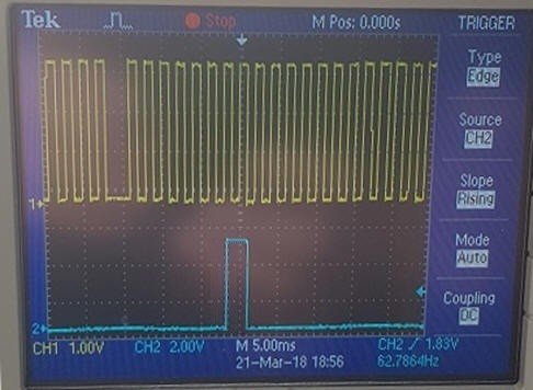
The image shows the dual-channel oscilloscope display, with the top trace showing the crankshaft reference point and the bottom trace showing the control signal from the MegaSquirt to the DIS coil. The control signal has a voltage of 5 volts (a logical 1) and lasts about 1.5 ms.
Ignition timing advance:
This project does not use knock sensors. While it is possible to process knock sensor information, merely installing a knock sensor does not suffice. Signal processing is complex. The knock signal must first be converted to a binary signal or an analog signal representing detonation strength.
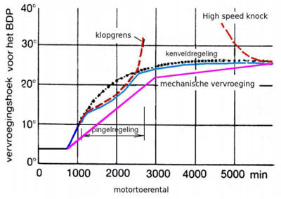
The conversion of engine vibrations to a knock signal is done by an interface circuit. This circuit is not present in the MegaSquirt II. Therefore, the choice was made to safely set the full-load and part-load advance, ensuring the engine does not enter the knocking range. The full-load advance curve must be established within the knock boundaries. Centrifugal and vacuum advance data from the conventional ignition is determined based on factory data from the engine manual. Points can be plotted on a graph (example in the image below).
The pink line indicates the original mechanical advance, partially linear due to the centrifugal weights’ mechanical construction. The black line represents the MegaSquirt field control; this line follows a curve. It’s crucial to avoid staying within the partial load and full load knock zones; thus, field control is limited in partial load (red line), and advance does not extend further in full load than with mechanical advance (red line). The actual field control proceeds according to the blue line.
First, the full load advance curve had to be filled out in the spark advance table. At higher rpm and lower load, more advance is needed. In part-load, the advance is added to the full-load advance. On page 7, the completed ignition advance table and the cold engine advance settings are displayed.
Throttle body:
The air/fuel supply was originally regulated by the carburetor. For the engine management system, the carburetor is replaced with a throttle body and four injectors mounted in the intake manifold. This achieves more precise and controlled injection than the carburetor, where an air/fuel mixture forms centrally in the manifold and distributes into four channels. The throttle is opened by a Bowden cable manually operated from the dashboard.
The MegaSquirt II does not support an electronically controlled throttle body. Therefore, Bowden cable operation is the only feasible option.
The throttle position is sent to MegaSquirt via a voltage. The voltage level depends on the throttle opening angle. The throttle position sensor is a potentiometer with a 5-volt supply (see image). Connection 3 and a ground connection 1 are necessary. The wiper (pin 2) takes a position on the resistance depending on the throttle opening. The wiper is thus connected to the throttle. When the wiper has to cover a small distance over the resistance (wiper points left), resistance is low. In the image, the wiper points to the right (ground side), indicating high resistance and low signal voltage.
In the applied throttle body, a 600mV voltage is present on the wiper when the throttle is closed and 3.9V when the throttle is fully open. The ECU receives this voltage and uses it to calculate the throttle opening angle. A rapid increase in opening angle indicates acceleration; the ECU responds with momentary enrichment called acceleration enrichment. The throttle position sensor does not determine mixture enrichment under different conditions; this is done using the MAP sensor.
Stepper motor test setup with simulator:
After MegaSquirt was hardware-modified, the breakout box could verify the reception of stepper motor control. The illumination of bi-color LEDs indicates control activation. Stepper motor control can be observed by monitoring color changes. The colors alternate between red and yellow. In the “Idle control” menu in TunerStudio, stepper motor data can be entered. Besides the type (4 wire), step count, including the position when the engine starts, can be specified. Additionally, the time duration for each step adjustment can be set.
The step count is partly dependent on coolant temperature; lower temperatures require a wider stepper motor opening. Steps relative to temperature can be set in a graph. The simulator verifies stepper motor control. Checking with the simulator first prevents issues during engine starting or running due to potential hardware or software problems. Since primarily coolant temperature and engine speed affect stepper motor opening, adjusting these potentiometers can verify correct control. The TunerStudio dashboard meter shows the adjustment in adjusted step numbers.
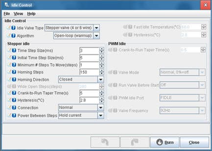
Stepper motor settings:
The image shows the settings screen for the stepper motor used for idle speed control.
Stepper motor steps were pre-set using an Arduino. Homing steps are also entered to move to its base position. The stepper motor is active during the warm phase (algorithm) and energizes coils during rest (hold current between steps).
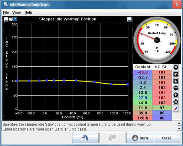
The stepper motor’s position depends on the coolant temperature. When starting a cold engine, the valve should be more open than with a warmed-up engine. The image below shows the settings screen to configure steps in relation to coolant temperature. When the engine is cold, the stepper motor remains fully open during idle. The stepper motor slightly closes during the warm-up phase.
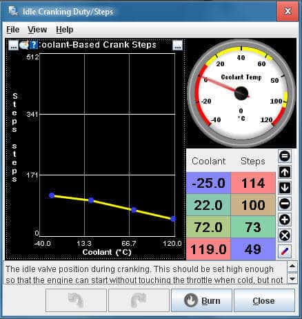
It is also possible to set the stepper motor position during engine starting based on the coolant temperature. This is called “Idle Cranking Duty/Steps.” The image below shows the settings screen.
Fuel pump circuit:
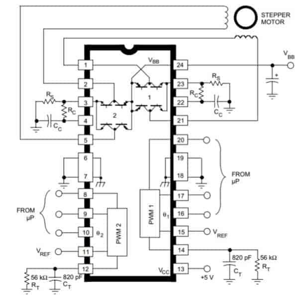
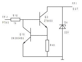
The MegaSquirt manages the fuel pump’s switching. Transistor Q19 in the image below protects transistor Q2 from excessive current. Excessive current can cause transistor burnout. As current increases through Q2’s collector-emitter part and R40, the saturation voltage at Q19’s base is reached. Transistor Q19 conducts, lowering the base-emitter voltage at Q2.
Connection FP-1 PTA0 is internally controlled by MegaSquirt. An input signal from the crankshaft position sensor (a Hall sensor or inductive sensor) is needed to drive the transistor circuit. If the signal is lost, such as during unexpected engine stall, the fuel pump power is immediately terminated.
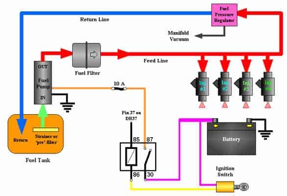
The transistor circuit’s output (FP1 OUT) connects to the fuel pump relay. Pin 85 of the relay is the output of the control current. When the relay is energized, the primary circuit (pins 30 and 87) is switched, providing operating voltage for the fuel pump.
An electronic fuel pump with 3 bar operating pressure is used. The fuel is directed through the fuel filter to the rail where pressure is exerted at the injectors’ inlets. A pre-calculated fuel amount will inject into the intake manifold upon MegaSquirt signal. Both MegaSquirt control and rail pressure determine the injected fuel amount.
Higher rail pressure results in greater fuel injection under the same control. Therefore, rail pressure must be adjusted based on intake manifold vacuum. The pressure difference (94P) should always remain 3 bar. The image shows the fuel system diagram. Pink, yellow, orange, and black lines depict electrical connections. The red line shows fuel supply, and the blue line fuel return.
Completing mechanical work:
The following three photos show the engine in the final phase of mechanical modifications.
Photo 1:
This side shows most installed parts. The dashboard for operation and MegaSquirt ECU are also visible here. A legend below the photo describes numbered parts. Click the pictures to enlarge them.
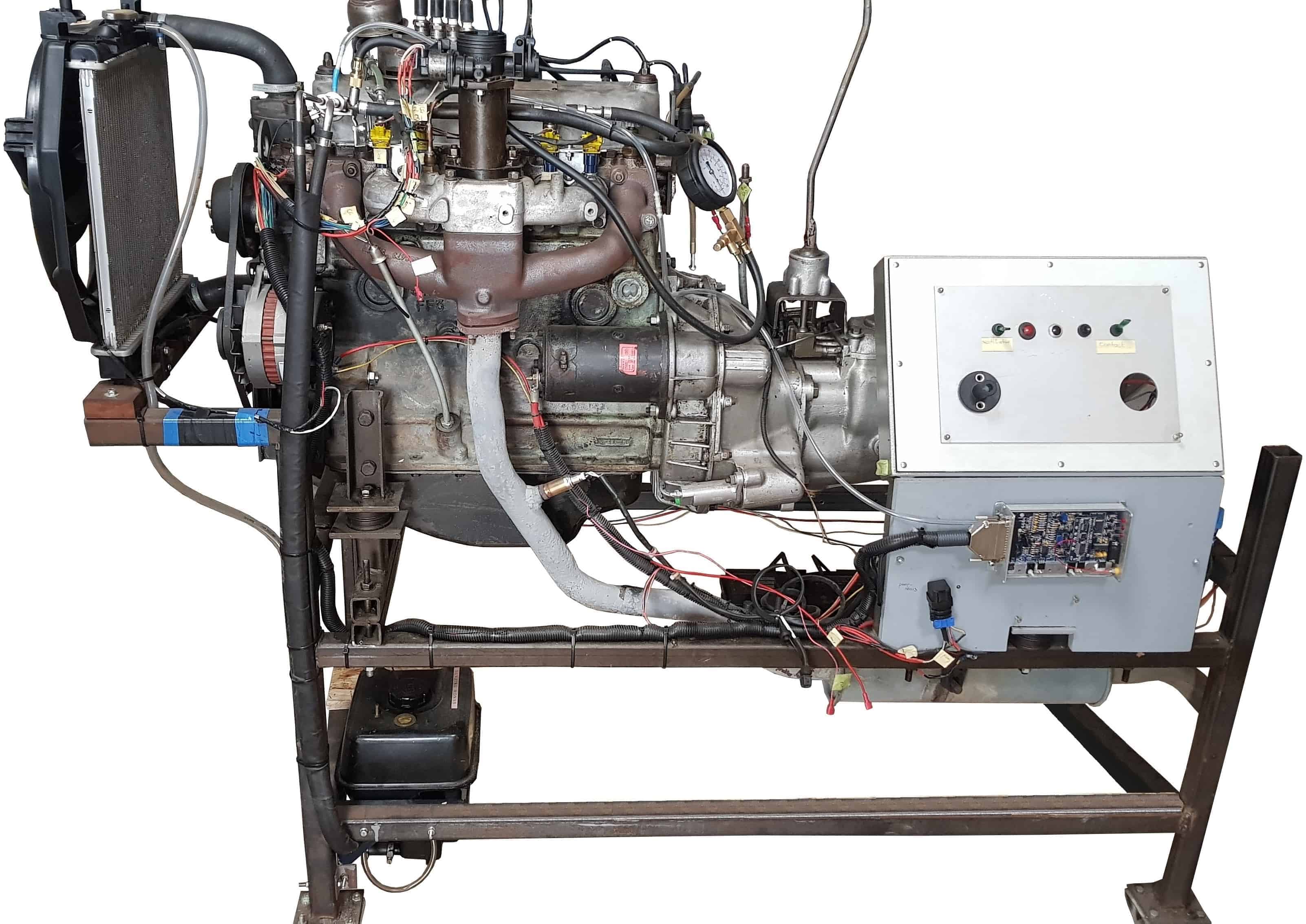
- Throttle;
- Fuel line for injectors;
- Connection tube from throttle to intake manifold;
- Fuel pressure gauge;
- Intake and exhaust manifolds;
- Dashboard with fan switch, dynamo and oil pressure lights, ignition switch, and ground switch;
- Vacuum hose for MAP sensor;
- Oxygen sensor;
- Fuel hoses (supply and return) bundled in a heat-shrink tube;
- Fuel pump/tank unit;
- Fuel pump relay;
- MegaSquirt;
- Exhaust muffler.
Photo 2:
This photo shows the other side of the engine. The carburetor (15) and conventional ignition (17) are visible. This classic ignition aims to spark test setup plugs (14). It’s functionless for the engine, but provides insight into how ignition worked in classic cars.
Number 20 indicates the transmission brake mechanism. A Bowden cable can engage the brake drum rod, braking the transmission’s output shaft. The transmission brake applies temporary load when a gear is engaged.
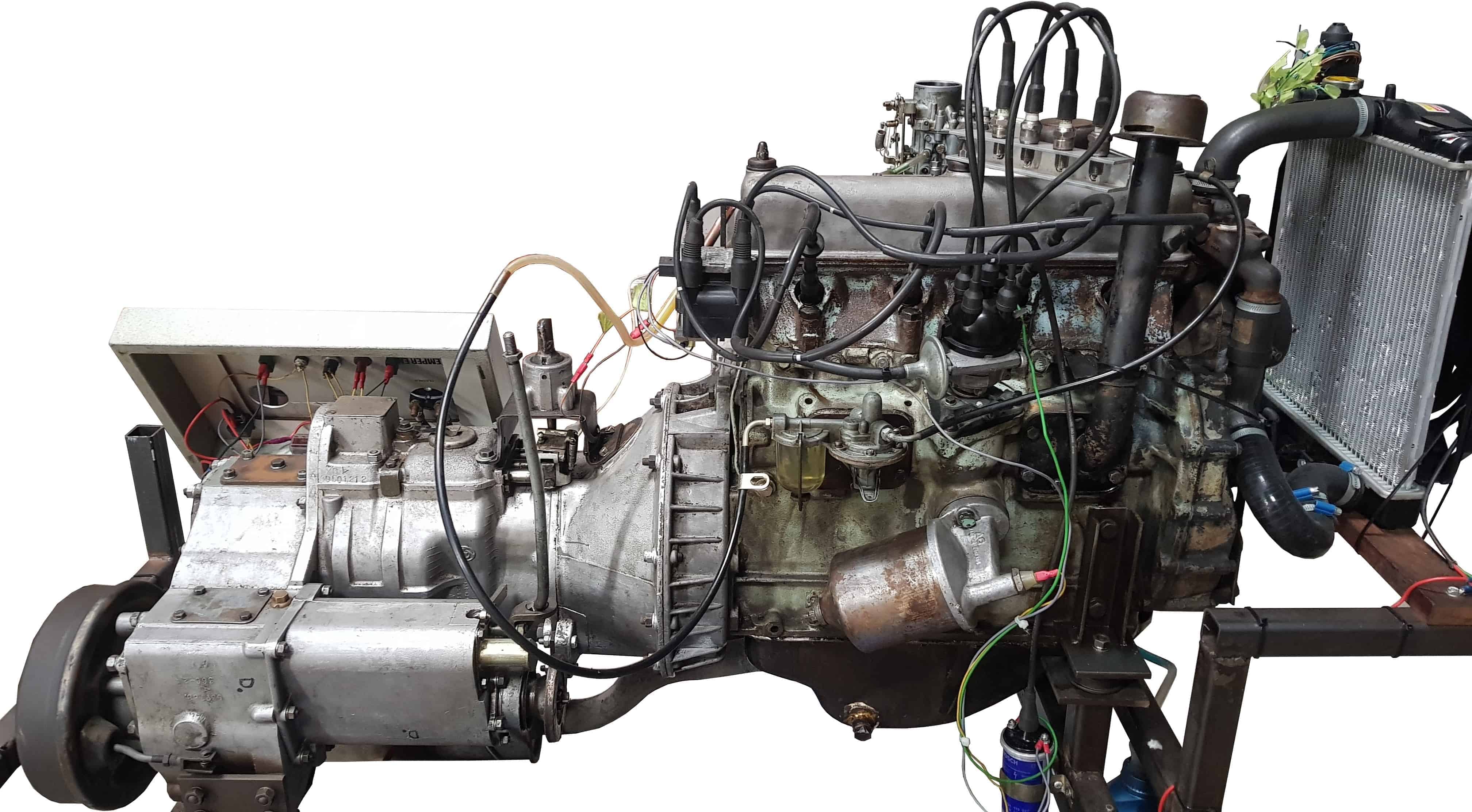
14. Mechanical distributor ignition test setup;
15. Carburetor;
16. DIS coil;
17. Mechanical distributor ignition with vacuum advance;
18. Dashboard’s rear;
19. Mechanical fuel pump;
20. Transmission brake mechanism;
21. Classic coil.
Photo 3:
The top view of the engine with the ignition and fuel rail test setup is clearly visible.
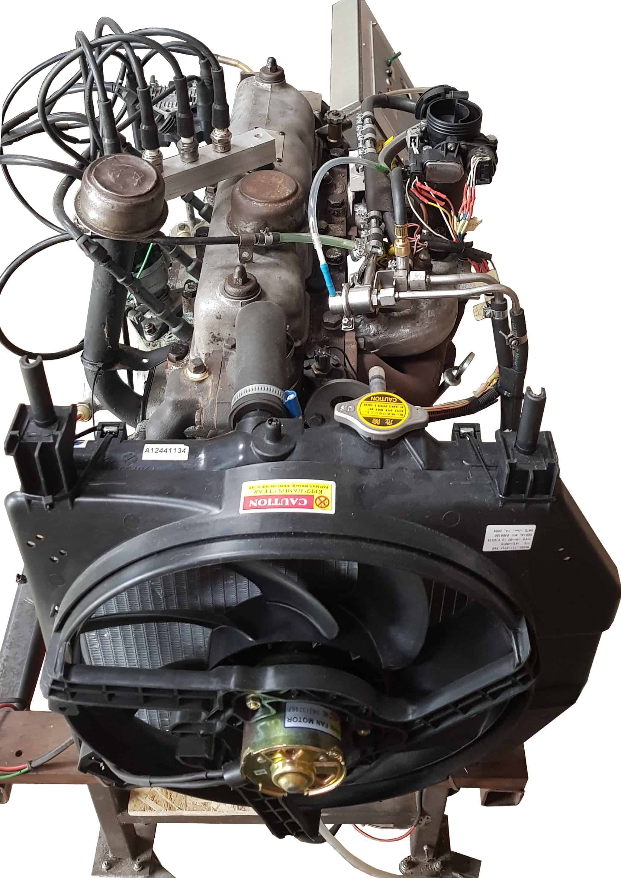
Mechanical modifications are completed. The engine cannot yet be started as some data must first be entered into the MegaSquirt.