Specific fuel consumption:
The fuel consumption of a vehicle is usually expressed in the number of kilometers driven per liter, for example: 1:15. In the vehicle documentation, the fuel consumption is often given in liters per 100 km, taking into account the driving conditions, such as the driving resistances that play a major role.
For technicians, it is interesting to know how much fuel it costs to deliver a certain power over a period of time. This consumption is expressed in kilograms of fuel per hour (B). When viewed per kilowatt, we talk about the specific fuel consumption (be), expressed in g/kWh.
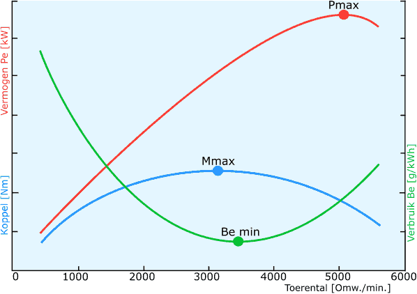
The specific fuel consumption can be included in the engine torque-power diagram of the vehicle. This diagram shows that the specific fuel consumption under full load conditions is the last at the point when the engine torque has just passed its maximum.
Engine efficiency:
The lowest specific fuel consumption is obtained under conditions where engine efficiency is highest. Power is expressed in Watts or Joules per second. The input power is the fuel’s thermal energy content, which is equal to the specific fuel consumption (be) * the delivered power (P) * the specific combustion heat (H).
Power diagram / contour plot:
In the testing phase of every (new) engine, a measurement for the specific fuel consumption takes place. This measurement is performed on an engine test bench or dynamometer under different RPMs with variable engine loads. The load is adjusted by pressing the throttle pedal progressively deeper, so the engine delivers a few kW more power at each step. This way, the entire RPM range is covered.
The diagram below shows the fuel consumption diagram, also known as the “contour plot.” The islands indicate fuel consumption in g/kWh. These lines (contour-shaped) connect the points where the specific fuel consumption is equal. The smallest island shows the lowest fuel consumption at an RPM of around 3000 RPM, namely 240 g/kWh. This is called the “sweet spot.” At such RPM and load, the engine is the most economical.
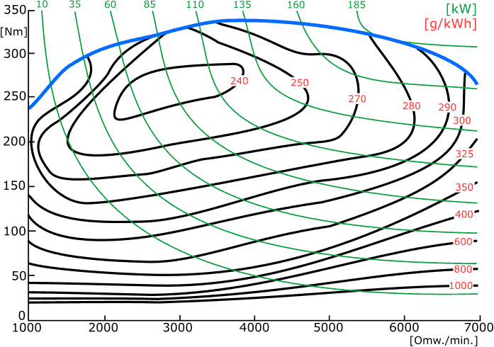
Explanation of the lines in the Contour plot:
- Vertical axis: torque in Nm;
- Horizontal axis: crankshaft speed;
- Blue line: the engine’s torque curve;
- Green lines: power lines in kW;
- Black islands: the consumption areas
In the (green) power lines, it is clear that with decreasing RPM, the torque (and thus the mean effective pressure) must increase to maintain the same power. Moreover, a decrease in fuel consumption is observed. The minimum fuel consumption of 240 grams per kWh is achieved at an RPM of around 3000 RPM at a delivered power of about 85 kW. The fuel consumption of this car is an average of 9 l/100 km.
This means that the engine is most economical when it has to deliver about 45% of the total power. At lower power outputs, the engine is inefficient: hardly any power is delivered, but all internal friction losses must be compensated. In practice, this can mean that the vehicle might be more fuel-efficient when driving at 120 km/h in 6th gear than at 90 km/h in 4th gear.
Power diagram with downsizing:
Until recently, manufacturers used engines with large displacements. The 6.0 (W-) 12-cylinder engine was the showpiece for the VAG group in, among others, the Audi A8, and the BMW M5 (E60) offered high performance with the naturally aspirated 5-liter V10 engine. Similarly, mid-range cars were equipped with relatively large displacements, e.g., a naturally aspirated 2.0-liter engine. Nowadays, manufacturers are searching for all possible ways to drastically reduce emissions without sacrificing performance. Increasingly, we see the displacement of engines getting smaller while a turbocharger provides good performance. An example of this can be seen in the VW Golf, where the 1.0-liter engine with a turbo outperforms and is more economical than an (older) 1.4-liter engine without a turbo:
- VW Golf V from 2005, displacement: 1.4 liters, power: 59 kW, consumption: 6.9 l/100 km (1:14.5);
- VW Golf VII from 2015, displacement: 1.0 liters, power: 85 kW, consumption: 4.5 l/100 km (1:22.2).
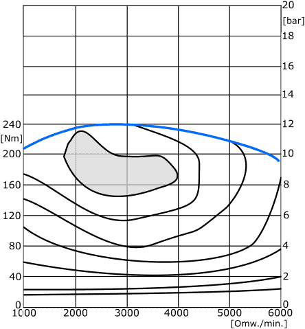
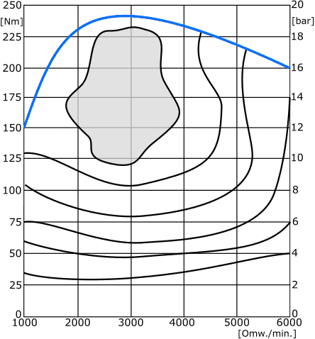
The contour plots below are of a naturally aspirated engine with a displacement of 2.5 liters and a turbocharged 1.6-liter engine. Both engines deliver a maximum torque of 240 Nm. The torque curve of the naturally aspirated engine is significantly flatter than that of the turbocharged engine around 3000 RPM. In both engines, maximum torque is achieved at approximately 3000 RPM, but we see that the average effective piston pressure (BMEP) is 7 bar higher in the turbocharged engine at the torque speed. A higher BMEP leads to fewer flow losses during gas exchange and higher efficiency.