Subjects:
- Picoscope general
- Picoscope: setting the voltage
- Picoscope: setting the time per division
- Picoscope: set trigger
- Picoscope: scale and offset
- Fluke: general
- Fluke: Turn on oscilloscope and connect test leads
- Fluke: Set Zero Line
- Fluke: Set voltage and time per division
- Fluke: Set Trigger
- Fluke: Enable or disable smooth feature
- Fluke: Enable Channel B
- Fluke: Measuring with the Clamp Meter
- Scope image of a duty cycle
- Scope image of a crankshaft and camshaft signal
- Scope view of an injector of an indirectly injected petrol engine
- Scope image of an injector of a common rail diesel engine
Picoscope general:
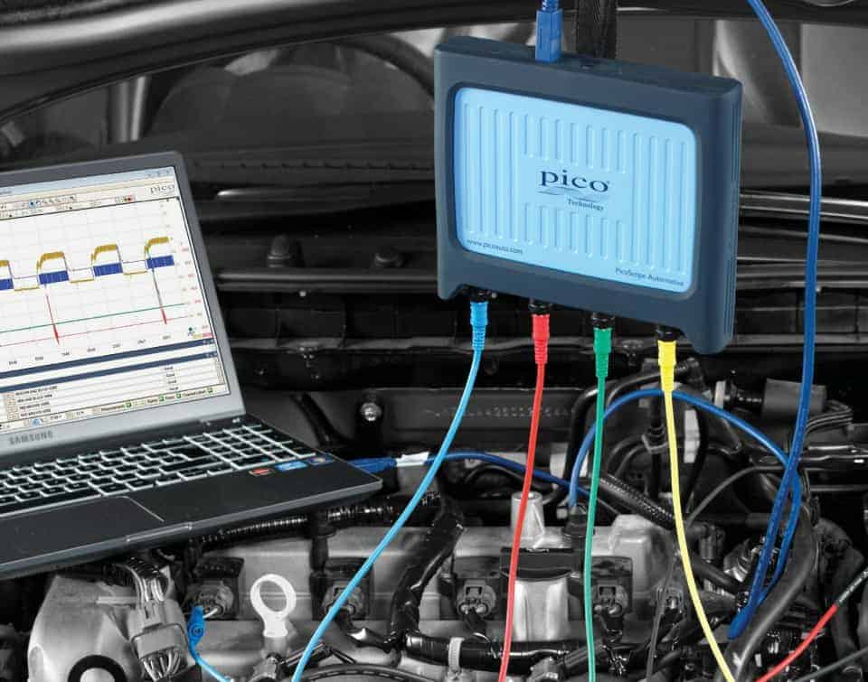
An oscilloscope is indispensable when making complex diagnoses. There are different variants of the oscilloscope: integrated in the readout equipment (eg with Snap-on), a “handheld” oscilloscope (Fluke, also described on this page) and linkable to a computer / laptop. The latter applies to the Picoscope. The hardware of this scope is built into a box that can be connected to a computer with the Windows or Macintosh operating system with a USB 3.0 (printer) cable.
On the computer we use the Picoscope software. The scope hardware enables various functions in the software; a more extensive (and more expensive) scope can therefore do more than an entry-level version. The Picoscope 2204a is available from €120 and is suitable for most automotive applications. The image shows the Automotive (4000 series) scope.
The basic settings for measurements with the Picoscope are described in the following paragraphs.
Picoscope: setting the voltage:
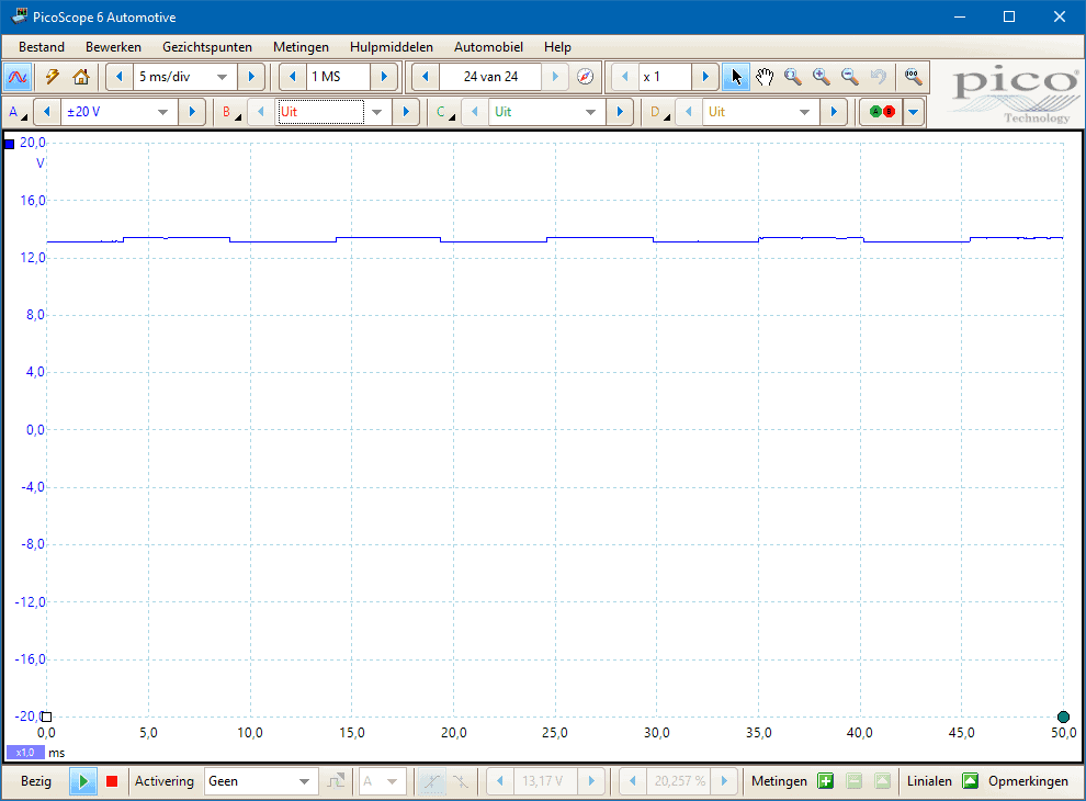
One of the settings to start measuring is to set the maximum voltage we expect to measure. After opening the program, the scale is set to “automatic”. This position can work against us if the height of the voltage changes significantly. In automotive applications, a 20 volt scale is sufficient in most cases. To set this up, we click on the button “20 V” under the red arrow. The menu that then opens shows the different options, ranging from 50 mV to 200 V. In this measurement, 20 V is selected. The maximum voltage to be measured is shown in the left Y-axis, indicated by the green arrow.
In this example, we are measuring a stable battery voltage of 12 volts.
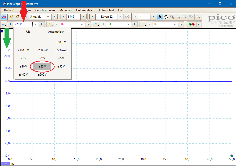
When the measured voltage is higher than the set voltage of (in this case) 20 volts, the message “channel overrange” will appear at the top of the screen. The voltage scale should then be increased. The arrows to the left and right of the menu button allow the voltage to be increased and decreased incrementally without entering the menu.
Picoscope: setting the time per division:
After we set the voltage to a maximum of 20 volts, the time can be set per division. To set this time, click on the time setting button (next to the red arrow). In the menu that appears we choose the desired time per division. 5 ms/div is circled in the image.
After clicking 5 ms/div you will see time at the bottom of the X-axis increasing each division, starting from 0,0 to 50,0. The time from 0 to 10 ms is circled in green in this example.
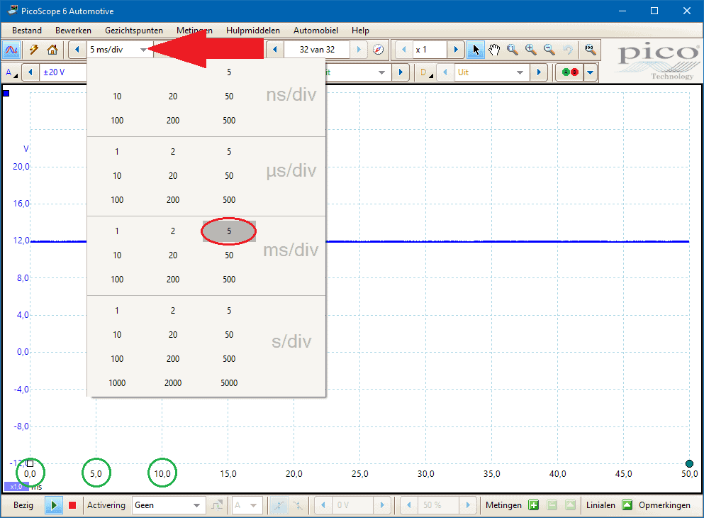
The time setting depends on which component, system or process we want to measure;
- battery voltage during cranking or a relative compression test: 1 second per division;
- signal from sensors and actuators: 10 to 100 ms/div.
During the measurement, the time base can be adjusted to show a correct signal on the screen.
Picoscope: set trigger:
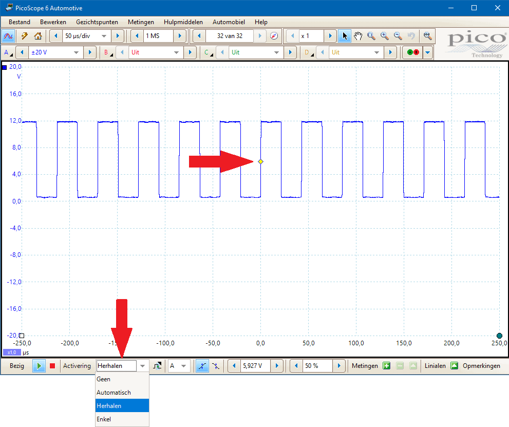
Constant voltages, such as the on-board voltage in the previous examples, can also be measured with a standard multimeter. Non-constant voltages, such as a strongly varying signal voltage from a sensor or a PWM control, cannot or can hardly be displayed by a voltmeter. In the case of a PWM or duty cycle, a voltmeter will indicate an average value. We measure such voltages with the oscilloscope. The scope image below is the PWM control of an interior fan. Without a trigger setting, the image will continue to jump across the screen.
The square-wave voltage constantly jumps across the screen. A change in the pulse width is difficult to detect. To fix the voltage on the image, but still measure real-time (no change is visible when pausing), we use the trigger. In the Picoscope software this is called “Activation”. This function can be found in the bottom bar of the screen. In this measurement, after Activation, it says: “None”. So no trigger is active.
The following image shows the image with the trigger enabled. We select (repeat). A yellow dot appears on the screen; this is the point of triggering. With the mouse we can move this point to any other place in the voltage range.
When measuring the signal, it may also be desirable to trigger on the negative edge; for example, when measuring the voltage image of an injector, because at that point the control starts. How to set it up: click on the “advanced triggers” button (red arrow in the image). A new screen opens where you can change the direction from “rising” to “descending” (blue arrow) at the “simple flank”. The trigger point in the signal is from that moment on the negative edge (green arrow).
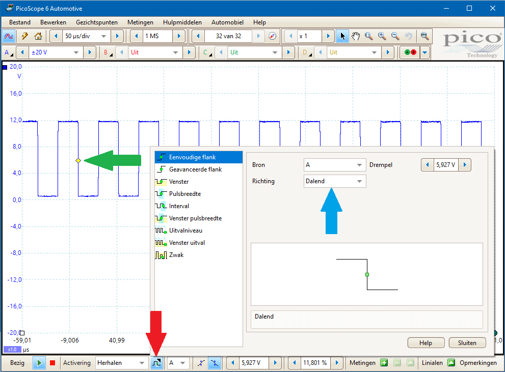
You can also set the trigger in many ways in this menu; eg a crankshaft signal contains 35 teeth and one missing tooth. This can be recognized by a space between the 35 pulses. With the function: “pulse width” the trigger can be set to the space formed by the missing tooth
The following example shows the voltage picture of an injector. Similar to the PWM control voltage of the passenger compartment fan in the previous example, this signal jumps across the screen.
After setting the trigger point, the signal is fixed on the screen (see figure below). The signal has a fixed starting point; where the injector is connected to ground, the control starts. Enrichment occurs during acceleration: the injector is opened for a longer time to inject more fuel. In that case, the ECU switches the injector to ground over a longer period of time. This can be seen in the scope image below.
When decelerating, the fuel injection stops: in that case the injector is not connected to ground. The voltage then remains constant (about 14 volts). Because we have set the trigger on the falling edge in this measurement, the deceleration cannot be clearly observed. Only after switching off the trigger do we see that the voltage remains 14 volts, but as soon as the injection is resumed, the image will jump across the screen again.
Picoscope: scale and offset:
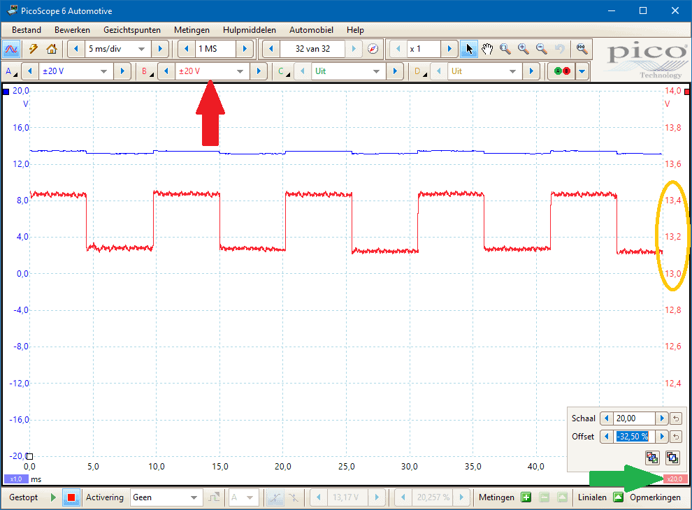
The block signal from an ABS sensor (Hall) has a small voltage difference. The scope image below shows the image measured directly on the ABS sensor. There is a circuit in the ABS control unit that increases the voltage difference. This scope image is not clear enough when diagnosing the ABS sensor. By changing the scale and offset, the signal can be magnified.
In the measurement below, channel B is connected to the same wire as channel A. The measurement is identical, but the different settings show the signal better. The green arrow indicates one of the places where you can change the scale and offset.
- The scale zooms in on the signal: we now measure the voltages within: 12 and 14 volts.
- The offset can be adjusted to get the signal at the right height. At an offset of 0%, the voltage on the Y-axis between 0 and 2 volts is visible.
Fluke in general:
An oscilloscope (abbreviated as scope) is a graphical voltmeter. The voltage is displayed graphically as a function of time. The scope is also very accurate.
The time can be set so small that signals from sensors such as the oxygen sensor or actuators such as an injector can be reproduced perfectly.
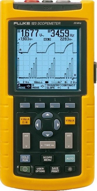
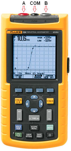
The image below is of a digital oscilloscope, which is used in car garages, in test and development rooms and in training courses. That can of course also be from a different brand, but then they often look almost the same. The operation is all pretty much the same. On top of the scope are a red and a gray connection. These are channels A and B. The ground connection is located in the middle.
Two measurements can be taken simultaneously on one screen (A and B separately). This can also be seen in this image. Measurement A is on top and measurement B is below. This makes it easy to compare signals from 2 different sensors. Channel A is used by default for a single measurement.
With the oscilloscope both direct voltage and alternating voltage can be measured. The sensors in the engine compartment, for example, provide a signal to the engine control unit. This signal can be checked by measuring with the oscilloscope. In this way it can be checked whether the sensor is defective or whether there is, for example, a broken cable or corrosion on the plug connections.
The battery voltage is measured in the picture. There are 7 boxes between the zero line (the black line at the bottom left) and the measured voltage (the thick line above A). Each square is called a division.
The voltage that must be set per division is set to 2 V/d (bottom left of the screen). That means that each square is 2 volts. Because there are 7 boxes between the zero line and the signal, it can be determined with a simple multiplication how many volts the indicated line is; 7*2 = 14 volts. The average voltage is also shown in the image (14,02 volts).
Fluke: Turn on oscilloscope and connect test leads:
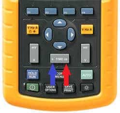
The green button at the bottom left of the device must be pressed to switch on the scope. To measure with the oscilloscope, the red test probe must be placed in channel A and the black probe must be placed in the COM connection.
To measure a signal, the red measuring pin (channel A, plus) must be placed on the signal connection of the sensor or in the correct place in the break-out box. The black test probe (COM) must be placed on a good ground point on the bodywork or the ground of the battery.
For a single voltage measurement, it is sufficient to use only channel A and the COM terminals.
When a measurement is to be performed where two voltage images are to be compared, channel B can be used. The probe must be plugged into connection B and channel B must be switched on in the oscilloscope.
The oscilloscope has the “AUTO” button. This function ensures that the oscilloscope itself finds the best settings for the input signal. The disadvantage of this function is that the correct signal is not always displayed; there is a danger that the oscilloscope changes the settings each time with a signal whose amplitude (the height of the signal) and the frequency (the width of the signal) change constantly. When two voltage images have to be compared with each other that both have different time settings, it can become very difficult. Therefore, it is better to manually set the oscilloscope and perform multiple measurements with the same settings. How to set up the oscilloscope manually is described in the following paragraphs.
Fluke: Set Zero Line:
After the oscilloscope is turned on, the zero line will often automatically set halfway down the screen. At a setting of 1 volt per division, the range will be only 4 volts. So there is only 4 volts in the screen. When a higher voltage is measured, the line will fall out of the picture.
In order to fit the entire voltage image into the screen, the zero line must be moved downwards. This can be seen in the image. The zero line is set here on the bottom line of the screen.
Now that the zero line is at the bottom and the oscilloscope is set to 1 V/d, a voltage of up to 8 volts can be displayed (8*1 = 8 v). This is fine for measuring the supply voltage or a signal from an active sensor (maximum 5 volts), but not enough for measuring higher voltages such as the battery voltage or the voltage across a lamp.
Fluke: Set voltage and time per division:
As described earlier, the number of volts per division must be set correctly in order for the voltage image to fit into the display. Setting the correct time per division is also important. The setting is described in this section.
If the number of volts per division is too low, the measurement will be out of the picture, but if the number of volts per division is too high, only a small signal will be visible. In the ideal measurement, the signal will be visible over the entire screen.
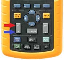
In the picture, the button marked mV and V adjusts the number of volts per division. Press mV to decrease the time per division and V to increase it.
By setting the time per division, the time in which measurements are taken can be changed. With a setting of 1 second per division (1 S/d), the line will move one square every second. This can also be seen in the voltage line; the line will move one division from left to right every second. Depending on the type of measurement, it is desirable to increase or decrease the time. When measuring the voltage profile of an injector, the time setting will have to be set lower than when measuring a duty cycle.
It can be increased by pressing the “s” on the left side of the “TIME” button. Lowering can be done with the “ms”. The time setting is the same for the A and B channels; a different time course cannot be set for channel A than for channel B.
Fluke: set trigger:
When measuring voltages such as battery voltage, no trigger is needed. The battery voltage (shown in paragraph “General”) is a straight line, counting the divisions between the zero line and the signal. The line is a constant. The height of the line will only change when the battery is charged or when a consumer is switched on. In the latter case, the line will get lower over time.
When measuring a sensor signal, the voltage line will not be constant. The height of the tension line will shift back and forth across the screen. Of course, the HOLD button can be used to pause the image so that the image can be viewed, but that is not ideal. The HOLD button must then be pressed at exactly the right moment. The second drawback is that no changes in the signal are shown because the image is frozen. The trigger function offers the solution for this. By setting the trigger, the voltage image on the screen will be held still at the set point. The measurement will then continue, so that the shape of the signal will change if the circumstances (for example the speed or temperature) change.
The symbols of the trigger are as follows:
Trigger for the rising edge. This trigger function keeps the tension image in place where it goes up.
Trigger for the falling edge. This is the inverted sign of the rising edge. This trigger function holds the voltage image when it goes down first.
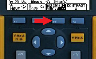
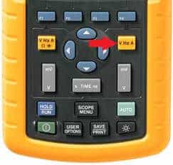
To move the trigger, press the F3 button (see picture). Move the trigger with the arrow keys up and down. Change the trigger from rising to falling edge with the left and right arrows.
In the bottom two images the same voltage image can be seen where the triggering was done in two different ways.
Trigger on the rising edge:
In the figure, the trigger is shown on the rising edge of the signal. The oscilloscope will therefore freeze the image as long as the sensor signal is being measured. If the trigger were not set, this signal would constantly scroll from left to right through the screen.
Trigger on the falling edge:
The trigger is set to the falling edge for the same measurement. This image clearly shows that the image is the same, but that the signal has shifted slightly to the left. This trigger function holds the image at the point where it goes down.
Obviously, the trigger is no way to pause the display. As soon as the measured object is switched off or when the signal changes, the signal in the image will change with it.
This can be seen in the image; the trigger is at the same point, but the horizontal tension line has become more than twice as long here. The voltage of 1,5 volts (1500mV) is now 110µs (microseconds) active instead of 45µs in the previous measurement.
Fluke: Enable or disable smooth feature:
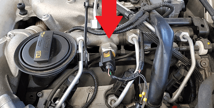
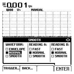
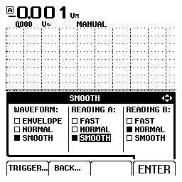
Because the oscilloscope is very accurate, there is always some noise on the image. This can be very disturbing, especially if you need to look closely at the voltage picture. To smooth the signal, the “smooth” function can be selected. The following measurement is made at the fuel pressure sensor. It is located on the fuel rail of the injectors of a common rail diesel engine (indicated by the red arrow in the picture below).
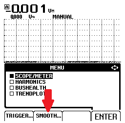
The Smooth function can be set by performing the following three steps:
Fluke: Enable Channel B:
When measuring signals, it may often be desirable to measure two signals relative to each other. This can be, for example, the camshaft signal and the crankshaft signal that are measured against time. The voltage profile of both sensors is then neatly displayed below each other from which conclusions can be drawn regarding the timing of the distribution.
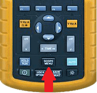
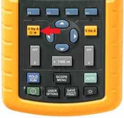
To enable channel B, the right yellow button on the oscilloscope must be pressed.
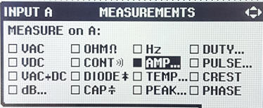
After a menu has appeared on the screen, the correct option can be selected with the arrow buttons. The option can be confirmed with the F4 button. At the top of the screen is F4 ENTER. Channel B can also be switched off again via this button.
The images below show the menu that appears after pressing the yellow button. In the left menu under B “OFF” is selected. It can be set to “ON” with the arrow keys. Furthermore, the option “Vdc” (DC voltage) must be selected. This can be seen in the right image. After each option has been confirmed with ENTER, this menu will disappear and you can start measuring with channel B.
Fluke: Measuring with the Clamp Meter:
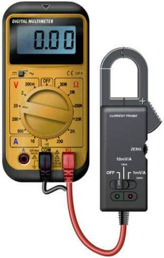
Only voltages can be measured with the oscilloscope. Even when current is measured with a current clamp, the oscilloscope will receive a voltage from the current clamp. This section explains how to measure with the clamp meter. To better understand it, here's an example of measuring with the multimeter.
The clamp meter can also be used in the multimeter. The current clamp contains a Hall sensor. The Hall sensor measures the magnetic field that flows through the measuring jaws of the current clamp. This magnetic field is converted into a voltage (up to 5 volts) in the clamp meter.
Where in the multimeter the internal fuse will break at a current higher than 10 Amperes, currents of hundreds of Amperes can be measured with the current clamp. The voltage transmitted by the clamp meter is 100 times smaller than the actual current. This is due to the conversion factor of 10 mV/A. This is also stated on the clamp meter.
Make sure that the current clamp is set in the first position, so not at 1mV/A (conversion factor 1000)
When the clamp meter is connected to the volt terminal of the multimeter, the clamp meter is switched on and calibrated until the multimeter reads 0 volts, the clamp meter can be placed around the cable of the sensor or actuator. Then, when reading the multimeter, the conversion factor must be taken into account; each millivolt the multimeter reads is actually 1 Ampere.
It is easy to remember that the value read must be multiplied by a factor of 100; when 0,25 volts is indicated in the display, the actual current is (0,25*100) = 25 amps.
When in another measurement the value 1,70 volts is shown in the display, the actual current strength is also one hundred times higher, so 170 amps.
Basically, the comma is moved two places to the right.
The previous example was measuring with the multimeter, because measuring with the scope might then be a little easier to understand. The same clamp meter can also be connected to the oscilloscope. The red and black leads of the clamp meter should be plugged into channel A (or B) and the COM terminal of the clamp meter.
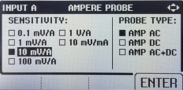
At this point, the oscilloscope is set to Ampere. First calibrate the clamp meter by turning the calibration knob so that the scope reads 0A.
When the clamp meter passes a voltage of 0,050 volts, the oscilloscope will convert this value itself by the factor of 100, because every 10 mV is in reality 1 Ampere. The display of the oscilloscope will now show 5 Ampere.
The clamp meter is very fast. With this function it is even possible to measure the current flow of an injector. With the two-channel function of the oscilloscope, for example, the voltage curve can be measured on channel A and the current curve on channel B. The voltage and current curves are neatly aligned.
Scope image of a duty cycle:
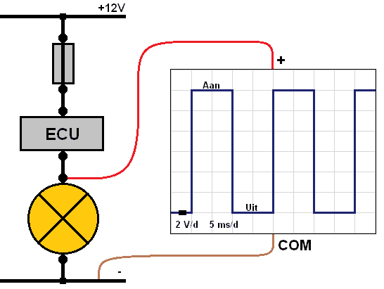
A duty cycle is used to regulate the current to a consumer. The image below shows a schematic of a lamp with the image of the oscilloscope on the right. The image shows that the voltage is continuously switched on and off. The voltage varies between 0 and 12 volts. Each square (division) is 2 volts, so six divisions means that the voltage is always 12 volts when the consumer is switched on and 0 volts when the consumer is switched off.
The plus cable of the oscilloscope is connected to the plus of the lamp. The ground cable is connected to the COM connection of the scope and the ground of the vehicle. Like the multimeter, the oscilloscope measures the voltage difference between the plus and minus cables. When the lamp is switched on, there is a voltage of 12 volts on the positive terminal of the lamp. The ground is always 0 volts, so when the lamp is switched on, the voltage difference is 12 volts. This can be seen in the scope image by the high line marked “on”.
When the lamp is turned off, the voltage difference will be 0 volts. Both the plus and minus cables will then measure 0 volts. In the screen of the oscilloscope this will also be visible on the line that is equal to the dash of the zero line. In the image above, this section also says “off”.
When measuring the duty cycle, it is necessary to take into account whether the consumer is connected positively or earth connected. The scope image will be the other way around. For more information, see the page duty cycle.
Scope image of a crankshaft and camshaft signal:
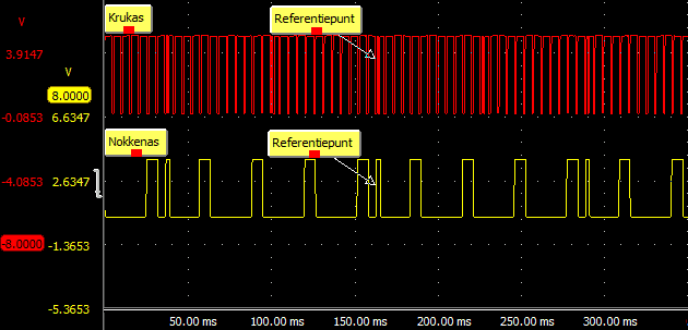
With the oscilloscope, several components can be measured relative to each other in the same time frame. This makes it possible to check whether sensors are giving a signal at the right time. An example can be seen in the scope image, where the crankshaft signal is compared with the camshaft signal.
By comparing these two signals, it is possible to check whether the timing of the distribution is still correct. More explanation about these signals can be found on the page crankshaft position sensor.
Scope image of an injector of an indirectly injected petrol engine:
With an actuator, such as a fuel injector, the current curve and the voltage curve can be displayed one below the other. In the scope image below, the current signal is yellow, and the voltage signal is shown in red. At the time 0.00 seconds, the injector is controlled by the ECU. The voltage then drops from 14 volts to 0 volts. The injector is therefore grounded. At that moment a current starts to flow; the yellow line will rise. At the time 1,00 ms the current is high enough to lift the injector needle from its seat; the injector opens and the fuel is injected. The injector is still controlled.
At the time 2.4 ms, the control by the ECU stops. The red line rises to 52 volts. This is the induction that takes place because the coil is charged. From that point on, both the voltage and current decrease. At the time 3,00 ms a bump can be seen in the voltage image. At this point, the injector needle closes. The injection is hereby terminated.
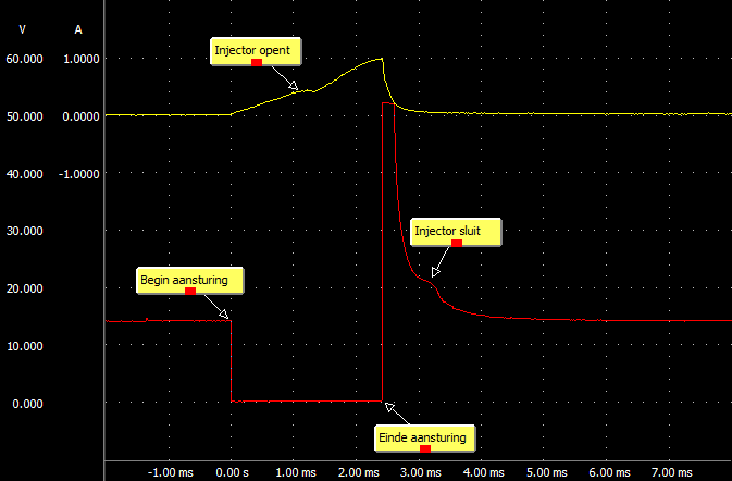
The actual injection time can therefore be seen in the scope image. The injection therefore starts and ends not between 0,00 and 2,4 ms, but between 1,00 and 3,00 ms. This has to do with the mass inertia of the injection needle. This is a mechanical part, in which the needle has to be moved against the spring force. When closing, it also takes 0,6 ms before the injector needle is pressed back onto its seat by the spring.
This scope image can be used to recognize whether the injector is still opening and closing. With a severely contaminated or defective injector, there are no bumps in the voltage and current signal. If these two points are flat, the control is OK, but there is no mechanical movement of the injector needle. This means that it can be ruled out that the control or wiring is defective and one can concentrate on the injector.
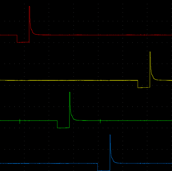
The scope image below shows four injector images one below the other. The red injector image is from cylinder 1, the yellow from cylinder 2, the green from cylinder 3 and the blue from cylinder 4. By placing these under each other, the firing order of a four-cylinder engine (1-3-4-2) can be seen .
Scope image of an injector of a common rail diesel engine:
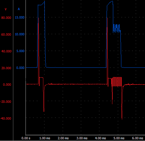
The scope image shows the voltage and current curve of an injector of a common rail diesel engine. Two injections take place in succession, namely the pre-injection and the main injection.
When the injector is switched on (during pre-injection), it is actuated very briefly with a voltage of 70 volts. The high voltage can be achieved thanks to a capacitor in the ECU. At that time, a current that rises to 20 amps is flowing. With this high voltage and high current, the injector needle is opened very quickly. Then the voltage is limited and kept at 14 volts. The current becomes a maximum of 12 amps. That is enough to keep the injector needle open. The voltage and current limitation is necessary to keep the heat development in the coil as low as possible. The control stops at the time 1,00 ms. The injector needle closes. This completes the pre-injection.
At the time 4,3 ms the main injection takes place. The voltage rises again to 65 volts and a current starts flowing again that increases to 20 amperes. The injection begins.
Subsequently, a voltage and current limitation takes place again between 4,60 and 5,1 ms. In this case, the injector needle is kept open. The amount of fuel injected can be regulated by driving the injector for a longer period of time.
See also the pages measuring instruments, measure with the multimeter en breakout box.
Measurements can also be made on the CAN bus. See there for the page measuring on the CAN bus system.